In my last article on expected goals I showed how to incorporate the distance from goal along the Y axis into the expected goal model using Pythagoras’ Theorem.
This all worked pretty well, giving us an r squared value of 0.95. However, while the r squared value was good there was still a flaw in the model we need to fix.
Better than Ronaldo
Eagle-eyed readers will have noticed that the fit of the curve broke down for very short distances, meaning the probability of scoring from zero metres was actually slightly above one. And as reader Benjamin Lindqvist commented, not even Ronaldo will score more than 100% of the time, not even from the goal line. Benjamin also had a good suggestion to improve this, adding an exponential decay function into the model to make it behave better around zero
Exponential Decay
If you aren’t familiar with exponential decay it basically means that a value decreases at a rate proportional to its current value. It’s a phenomenon that crops up fairly frequently in science and the natural world. For example, air pressure decays exponentially as you go higher up into the Earth’s atmosphere and radioactivity decreases exponentially over time.
A general equation for exponential decay is shown in Figure 1, where Y(t) is the value at time t, a is the starting value, k is the decay constant and t is time.
So how do we apply this to football? Well, the first thing to do is replace time with metres and assume that the probability of scoring a goal decreases exponentially based upon the distance from goal the shot is taken from.
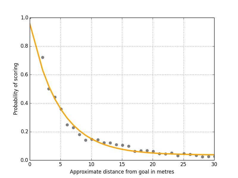
Next we need to find the correct value for the decay constant as this controls the shape of the curve. Rather than doing this manually through trial and error, we can use something such as R’s optim function to find it for us. We can also tweak the equation to add in a multiplier for the independent variable and an intercept as found in a traditional regression model giving us the fit shown in Figure 2.
Notice how the orange line now hits the Y axis just below 1.0? This fixes the problem we had before where it was possible to score more than one goal from a single shot. In fact, if you’re standing on the goal line the model now predicts around 0.96 expected goals, so very likely to score but with a small chance of screwing up (yes Edin Džeko I’m looking at you).
The new curve fit also pushes the r squared value up to 0.9883, meaning 98.83% of the variance for the probability of scoring from a shot can be accounted for using just distance from goal along the X and Y axes.
The final equation (Figure 3) is slightly more complicated now but it’s still pretty simple to use.
where:
and dx, dy are the difference between the x coordinates and y coordinates in metres for the shot location and the goal location.
As ever, let me know what you think!


